Quick Overview#
This tutorial will help you get started with basic usage of the FanInSAR library. We will cover the following topics:
How to initialize a dataset
How to query values from dataset by given points/bounding boxes/polygons
How to operate time series processing (e.g., unwrapping error correction, NSBAS inversion, etc.)
How to save the processed results into tiff/kml(kmz) files
Imports#
Customarily, we import FanInSAR as follows:
from pathlib import Path

import numpy as np

import faninsar as fis
from faninsar import NSBAS, cmaps, datasets, query
Load InSAR datasets#
FanInSAR provides a series of Datasets to load well-known InSAR products. Here we will use the HyP3S1 for example, which is used to load the HyP3 Sentinel-1 frame dataset.
Tip
If Datasets provided by FanInSAR do not meet your requirements, you can also create your own dataset class following the tutorial: Custom Interferometric Datasets
Initialize a dataset#
To initialize the HyP3S1 class, you only need to provide the root directory of the HyP3 data. All unwrapped interferogram and coherence files stored in the root directory, including the subdirectories, will be automatically scanned.
root_dir = Path("/Volumes/Data/GeoData/YNG/Sentinel1/Hyp3/descending_roi/")
ds_unw = datasets.HyP3S1(root_dir, fill_nodata=True)
Tip
You can also directly provide the
paths_unwandpaths_coharguments to specify the paths of the unwrapped and coherence files. In this case, theroot_dirargument will be ignored.Only common pairs of the unwrapped interferogram and coherence files will be used. The rest of the files will be ignored automatically.
More initialization parameters
Below are the common parameters to initialize a dataset:
crs, res, resampling:
If the dataset files are not aligned with the specified
crs(Coordinate Reference System) orres(resolution), the warp process, such as resampling and reprojection, will be performed to align the dataset files with the specifiedcrsandresautomatically. (Warping upon loading section provides some examples of usage)The
resamplingparameter is employed to define the resampling algorithm used in the warp process. The default value isResampling.nearest. More resampling algorithms can be found Resampling.
fill_nodata: If
True, the nodata values in raster files will be interpolated using inverse distance weighting method provided by the rasterio.fill.fillnodata().roi: region of interest, which defines the specific area to be loaded from the dataset. If left as
None, the combined boundary of all files within the dataset will be utilized.verbose: Enabling
verbose=Truewill display the dataset processing information. To suppress this output, set the parameter toFalse.
Interferogram dataset#
HyP3S1 is a subclass of PairDataset and provides the same functionalities/properties as PairDataset. You can view interferogram file by directly calling files property. The file paths and whether the file is valid or not will be displayed in the DataFrame format.
ds_unw.files
| paths | valid | |
|---|---|---|
| 0 | /Volumes/Data/GeoData/YNG/Sentinel1/Hyp3/desce... | True |
| 1 | /Volumes/Data/GeoData/YNG/Sentinel1/Hyp3/desce... | True |
| 2 | /Volumes/Data/GeoData/YNG/Sentinel1/Hyp3/desce... | True |
| 3 | /Volumes/Data/GeoData/YNG/Sentinel1/Hyp3/desce... | True |
| 4 | /Volumes/Data/GeoData/YNG/Sentinel1/Hyp3/desce... | True |
| ... | ... | ... |
| 2745 | /Volumes/Data/GeoData/YNG/Sentinel1/Hyp3/desce... | True |
| 2746 | /Volumes/Data/GeoData/YNG/Sentinel1/Hyp3/desce... | True |
| 2747 | /Volumes/Data/GeoData/YNG/Sentinel1/Hyp3/desce... | True |
| 2748 | /Volumes/Data/GeoData/YNG/Sentinel1/Hyp3/desce... | True |
| 2749 | /Volumes/Data/GeoData/YNG/Sentinel1/Hyp3/desce... | True |
2750 rows × 2 columns
We keep the same API with rasterio for the dataset, so you can use directly access the resolution, bounds, and other properties of the dataset just like using rasterio.
Important
The res, crs, dtypes and nodata parameters used during dataset initialization represent the output properties of the dataset, which the user can specify. This is a fancy feature of FanInSAR, enabling warping upon loading the dataset (See Warping upon loading for more details). Note that these properties may differ from the actual properties of the raster files themselves.
print(f" res: {ds_unw.res}\n bounds: {ds_unw.bounds}\n crs: {ds_unw.crs}\n dtype: {ds_unw.dtype}\n nodata: {ds_unw.nodata}")
 res: (40.0, 40.0)
 bounds: BoundingBox(left=443501.82025355106, bottom=4263758.21737383, right=536101.820253551, top=4335118.21737383, crs=EPSG:32647)
 crs: EPSG:32647
 dtype: float32
 nodata: 0.0
All valid unwrapped interferogram and coherence files will be indexed, and a corresponding Pairs instance will be created automatically. This feature eliminates the need to manually manage file names, as the pairs are generated based on the file names.
You can access the pairs through the pairs property, which supports advanced indexing and filtering operations, similar to pandas (see Indexing/Filtering Pairs for more details).
ds_unw.pairs
          Pairs
        primary  secondary
0    2015-11-12 2015-12-06
1    2015-11-12 2015-12-30
2    2015-11-12 2016-01-23
3    2015-11-12 2016-02-16
4    2015-11-12 2016-03-11
...         ...        ...
2745 2023-03-23 2023-08-14
2746 2023-03-23 2023-09-07
2747 2023-04-04 2023-08-14
2748 2023-04-04 2023-09-07
2749 2023-08-14 2023-09-07

[2750 rows x 2 columns]Coherence dataset#
The coherence dataset can be accessed by the coh_dataset property of the HyP3S1 object. The coherence dataset is also a PairDataset object, so you can access the properties of the coherence dataset just like the unwrapped interferograms.
ds_coh = ds_unw.coh_dataset
ds_coh.pairs
          Pairs
        primary  secondary
0    2015-11-12 2015-12-06
1    2015-11-12 2015-12-30
2    2015-11-12 2016-01-23
3    2015-11-12 2016-02-16
4    2015-11-12 2016-03-11
...         ...        ...
2745 2023-03-23 2023-08-14
2746 2023-03-23 2023-09-07
2747 2023-04-04 2023-08-14
2748 2023-04-04 2023-09-07
2749 2023-08-14 2023-09-07

[2750 rows x 2 columns]Query values by Points/Boxes/Polygons#
FanInSAR provides a Queries module, which defines a series of classes to query/sample values from the dataset by given points, bounding boxes, or polygons and store the results of the queries.
Define queries#
Query types in FanInSAR
There are four types of queries in the query module: Points, BoundingBox, Polygons, and GeoQuery:
Points: A collection of points, can be used to sample multiple pixel values from GeoDataset.
BoundingBox: A bounding box, can be used to sample rectangular region values from GeoDataset.
Polygons: A collection of polygons, can be used to sample multiple polygon values from GeoDataset.
GeoQuery: A combination of
Points,BoundingBox, andPolygons. It is highly recommended if you want to sample values using multiple query types simultaneously.
Below is an example of how to define a GeoQuery containing both reference points and a bounding box
# initialize a Points from a shape file, which contains reference points
ref_file = "/Volumes/Data/GeoData/YNG/ARPs.geojson"
ref_points = query.Points.from_shapefile(ref_file)

# define a bounding box for the region of interest
roi = query.BoundingBox(
    98.86517887, 38.78630936, 98.90998476, 38.83929150, crs="EPSG:4326"
)

# define a GeoQuery, which is a combination of a bounding box and a set of reference points
geo_query = query.GeoQuery(boxes=roi, points=ref_points)
Tip
You can provide the crs parameter to specify the coordinate reference system of the query.
The query will be automatically reprojected to the dataset’s crs if the crs is not the same as the dataset’s crs.
If the crs is not provided, It will be set to the same as the dataset by default.
Query values by GeoQuery#
There are two methods to query values from a dataset: using [] and using the query() method.
Query by []#
This is a direct querying method, suitable when you only need to retrieve all valid pairs.
unw_sample1 = ds_unw[geo_query]
Loading Interferogram Files: 100%|██████████| 2750/2750 [01:11<00:00, 38.45 files/s]
Query by query() method#
This method offers more flexibility, allowing you to query the values of a subset of pairs by specifying the pairs parameter. This means you can easily modify the SBAS network by specifying the pairs you want to query.
Strategy for selecting pairs
In this tutorial, two components are considered in the selection of interferometric pairs in the SBAS network:
Pairs(days<=60): All interferometric pairs with temporal baselines of lease than 60 days.
Pairs(nearest winters): All available interferometric pairs between adjacent winters are constructed. Specifically, for each winter, all acquisitions from January 1st to March 31st for each year are selected, during which period the active layer is typically completely frozen.
Adding pairs that link to the nearest winters can help to mitigate the cumulative bias in deformation time series caused by multi-looking and spatial filtering operations in SBAS.
Reference
Systematic phase biases in InSAR time series can be caused by the multi-looking and spatial filtering operations in SBAS:
Ansari, H., De Zan, F., Parizzi, A., 2021. Study of Systematic Bias in Measuring Surface Deformation With SAR Interferometry. IEEE Transactions on Geoscience and Remote Sensing 59, 1285–1301. https://doi.org/10.1109/TGRS.2020.3003421
Zheng, Y., Fattahi, H., Agram, P., Simons, M., Rosen, P., 2022. On Closure Phase and Systematic Bias in Multilooked SAR Interferometry. IEEE Transactions on Geoscience and Remote Sensing 60, 1–11. https://doi.org/10.1109/TGRS.2022.3167648
Maghsoudi, Y., Hooper, A.J., Wright, T.J., Lazecky, M., Ansari, H., 2022. Characterizing and correcting phase biases in short-term, multilooked interferograms. Remote Sensing of Environment 275, 113022. https://doi.org/10.1016/j.rse.2022.113022
For the permafrost regions, The phase biases can be effectively mitigated by adding interferometric pairs that linking the nearest winters:
Fan, C., Liu, L., Zhao, Z., Mu, C., 2025. Pronounced underestimation of surface deformation due to unwrapping errors over tibetan plateau permafrost by sentinel-1 InSAR: identification and correction. J. Geophys. Res.: Earth Surf. 130, e2024JF007854. https://doi.org/10.1029/2024JF007854
pairs = ds_unw.pairs

# select the pairs within a specific time period
period_mask = pairs.where(pairs["2017":"2023-04"], return_type="mask")
# prepare the mask for the two types of pairs
mask_nearest_winter = (
    period_mask
    & (pairs.days > 180)
    & (pairs.days < 360 + 180)
    & (pairs.primary.month.map(lambda x: x in [1, 2, 3]))
    & (pairs.secondary.month.map(lambda x: x in [1, 2, 3]))
)
mask_60 = (pairs.days <= 60) & (period_mask)

# combine the two masks to select the pairs
pairs_mask = mask_60 | mask_nearest_winter
pairs_used = pairs[pairs_mask]

# query the interferogram and coherence files with the selected pairs
unw_sample2 = ds_unw.query(geo_query, pairs=pairs_used)
coh_sample2 = ds_coh.query(geo_query, pairs=pairs_used)
Loading Interferogram Files: 100%|██████████| 1090/1090 [00:21<00:00, 51.71 files/s]
Loading Coherence Files: 100%|██████████| 1090/1090 [00:27<00:00, 39.45 files/s]
Results of queries#
Properties of query results
QueryResult class is used to store the query results. It contains the following four properties:
points: Result of the
Pointsquery.boxes: Result of the
BoundingBoxquery.polygons: Result of the
Polygonsquery.query: The original
GeoQueryinstance used to query the dataset.
check the query results for [] method
unw_sample1
QueryResult(
    points=PointsResult(files:2750, points:107),
    boxes=BBoxesResult(files:2750, height:147, width:97),
    polygons=None,
    query=GeoQuery(points=Points(count=107, crs='EPSG:4326'), boxes=[1 BoundingBox], polygons=None)
)
# Following steps will only use unw_sample2 for demonstration
del unw_sample1
check the query results for query() method
unw_sample2
QueryResult(
    points=PointsResult(files:1090, points:107),
    boxes=BBoxesResult(files:1090, height:147, width:97),
    polygons=None,
    query=GeoQuery(points=Points(count=107, crs='EPSG:4326'), boxes=[1 BoundingBox], polygons=None)
)
Tip
For each query type, the masked numpy array values are stored in the data property, and the corresponding dimensions are stored in the dims property.
We typically take the mean phase values of multiple reference points as the final reference point value. In FanInSAR, re-referencing process can be easily achieved by the code below:
# calculate the mean phase values of multiple reference points
ref_values = unw_sample2.points.data.mean(axis=1)

# re-referencing the phases
unw_img = unw_sample2.boxes.data - ref_values[:, None, None]
# load the coherence data
coh_img = coh_sample2.boxes.data
Time-series processing#
Note
This tutorial only demonstrates the basic usage of the FanInSAR library. The atmospheric correction is not included in this tutorial. In practice, however, the atmospheric correction is typically necessary to obtain accurate surface deformation time series.
Unwrapping error correction#
Here, we will demonstrate how to correct the unwrapping errors in the interferograms using the method presented in the following reference:
Reference
Poster: Fan, C., Liu, L., Mu, C., 2023. “Does InSAR Time Series Using C-band Sentinel-1 Data Underestimate Surface Deformation Over Permafrost Regions on Qinghai-Tibetan Plateau?” Presented at the AGU23, AGU. https://agu23.ipostersessions.com/default.aspx?s=7E-2A-74-4D-47-0B-85-B9-6A-ED-25-42-9B-4A-48-87
Paper: Fan, C., Liu, L., Zhao, Z., Mu, C., 2025. Pronounced underestimation of surface deformation due to unwrapping errors over tibetan plateau permafrost by sentinel-1 InSAR: identification and correction. J. Geophys. Res.: Earth Surf. 130, e2024JF007854. https://doi.org/10.1029/2024JF007854
In this tutorial, the interferograms with temporal baselines less than 12 days are treated as the reliable edge pairs, and are used to correct the unwrapping errors in the diagonal pairs, which temporal baselines are longer than 12 days.
First, we need to generate loops with given edge pairs. This can be easily achieved by the faninsar.Pairs.to_loops method of the Pairs class by specifying the edge_pairs parameter.
# filter the edges pairs with temporal baseline less than 12 days
edge_pairs = pairs_used[pairs_used.days <= 12]

# get the loops with edges pairs
loops = pairs_used.to_loops(max_acquisition=6, edge_pairs=edge_pairs)
loops
Loops(
    loops=664,
    pairs=840,
    edge_pairs=176,
    diagonal_pairs=664
)
Then, we can correct the unwrapping errors in the diagonal pairs using the un-closure phases of the loops. This can be done by the calculate_u() function in the NSBAS module.
# reshape the unw_img and coh_img to 2D array (n_img, n_pixel) for calculation
n_img, n_row, n_col = unw_img.shape
unw = unw_img.reshape(n_img, -1)
coh = coh_img.reshape(n_img, -1)

# =============================================================================
# there are cases that not all the pairs are used in the loops
# so we need to select the pairs that are used in the loops
# =============================================================================

idx = pairs_used.where(loops.pairs)
unw_used = unw[idx]

# calculate the correction term u
u = np.zeros_like(unw, dtype=np.float32)
u[idx] = np.round(NSBAS.calculate_u(loops, unw_used))

# calculate the corrected interferometric phases
unw_c = unw - 2 * np.pi * u
NSBAS inversion chain#
Convert phase to deformation#
FanInSAR provides a PhaseDeformationConverter class to convert values between phase and deformation.
To initialize the PhaseDeformationConverter class, you need to provide an instance of either Wavelength or Frequency of the radar. These two parameters are typically the built-in properties of the well-known InSAR dataset classes.
ds_unw.wavelength, ds_unw.frequency
(Wavelength(data=55.46576466234968, unit='mm'),
 Frequency(data=5.405, unit='GHz'))
You can call the phase2deformation() method to convert the unwrapped phase to deformation in millimeters (mm).
# initialize a PhaseDeformationConverter instance with the frequency of Sentinel-1
pdc = fis.PhaseDeformationConverter(ds_unw.wavelength)

# convert the unwrapped phases to deformation
d = pdc.phase2deformation(unw)
d_c = pdc.phase2deformation(unw_c)
Note
In FanInSAR, deformation/displacement is referenced to Earth, resulting in inverted signs when referring to radar measurements. Specifically, negative values indicate movement away from the radar (e.g., subsidence), while positive values signify movement towards the radar (e.g., uplift).
Mask low coherence pixels#
Before the NSBAS inversion, we typically mask the pixels with low coherence values. This can be done by numpy.ma module. Following is an example of how to mask the pixels with coherence values less than 0.3.
t_coh = 0.3

d = np.ma.array(d, mask=coh < t_coh)
d_c = np.ma.array(d_c, mask=coh < t_coh)
Tip
the masked numpy array MaskedArray still stores the raw data, and can be accessed by the data property.
Define time series model#
Time-Series Models module provides a series of time series models. Here we use the AnnualSemiannualSinusoidal model as an example.
Tip
If None of the models in the Time-Series Models module meet your requirements, you can define your own time series model following the tutorial: Custom Time Series Models.
ts_model = NSBAS.AnnualSemiannualSinusoidal(pairs_used.dates, unit="year")
Initialize a time series model
For the mathematical models, you typically only need to provide the
datesof acquisitions to initialize a time series model.For the more complex physical models, you need to check the specific initialization parameters in the documentation. For example, the FreezeThawCycleModelWithVelocity model requires the
datesandftcparameters to be specified.
Operate NSBAS inversion#
Theory of NSBAS inversion
The objective of the SBAS/NSBAS inversion is to estimate the m for the equation:
where:
m (model domain): a vector of
N-1incremental deformations of adjacentNSAR acquisitions (and the time series model parameters for NSBAS inversion).d (data domain): a vector of the deformation/(unwrapped phases) of interferograms.
G: a design matrix that maps the values in data domain
dto the model domainm.
The least squares solution is typically used to solve the equation (1) to estimate the m.
Reference
Following papers are recommended for understanding the NSBAS inversion method:
López-Quiroz, P., Doin, M.-P., Tupin, F., Briole, P., Nicolas, J.-M., 2009. Time series analysis of Mexico City subsidence constrained by radar interferometry. Journal of Applied Geophysics, Advances in SAR Interferometry from the 2007 Fringe Workshop 69, 1–15. https://doi.org/10.1016/j.jappgeo.2009.02.006
Fan, C., Mu, C., Liu, L., Zhang, T., Jia, S., Wang, S., Sun, W., Zhao, Z., 2025. Time-series models for ground subsidence and heave over permafrost in InSAR processing: a comprehensive assessment and new improvement. ISPRS J. Photogramm. Remote Sens. 222, 167–185. https://doi.org/10.1016/j.isprsjprs.2025.02.019.
FanInSAR streamlines the process of generating the design matrix G and data vector d through the NSBASMatrixFactory class. After initializing this class, you can directly access the design matrix G and data vector d as properties.
matrix_factory = NSBAS.NSBASMatrixFactory(d, pairs_used, ts_model)

print(matrix_factory.d.shape, matrix_factory.G.shape)
(1273, 14259) (1273, 188)
FanInSAR also streamlines the process of solving the least squares problem to estimate the m through the NSBASInversion class. After initializing this class, you can directly perform the inversion by calling the inverse() method.
sbas_inverse = NSBAS.NSBASInversion(matrix_factory, device="cpu")
inc, params, residual_pair, residual_tsm = sbas_inverse.inverse()

# calculate the cumulative deformation by the incremental deformation
cum = np.cumsum(inc, axis=0)
# insert a zero row for the first acquisition
cum = np.insert(cum, 0, 0, axis=0)
NSBAS inversion: 100%|██████████| 1297/1297 [00:05<00:00, 259.09Batch/s]
Tip
FanInSAR uses the
PyTorchlibrary as the backend for the computation. Therefore, you can easily switch the computation between theGPUandCPUby specifying thedeviceparameter. See the torch.device for more information.Low-level functions for the least squares problem, such as censored_lstsq() and batch_lstsq(), are also provided in the NSBAS.inversion module.
perform NSBAS inversion for the unwrapped phases that not been masked by the coherence values for comparison.
matrix_factory = NSBAS.NSBASMatrixFactory(d.data, pairs_used, ts_model)
sbas_inverse = NSBAS.NSBASInversion(matrix_factory, device="cpu")
inc_r, params_r, residual_pair_r, residual_tsm_r = sbas_inverse.inverse()
cum_r = np.cumsum(inc_r, axis=0)
cum_r = np.insert(cum_r, 0, 0, axis=0)
NSBAS inversion: 100%|██████████| 1189/1189 [00:04<00:00, 240.23Batch/s]
perform NSBAS inversion for the corrected unwrapping phases for comparison.
matrix_factory = NSBAS.NSBASMatrixFactory(d_c, pairs_used, ts_model)
sbas_inverse = NSBAS.NSBASInversion(matrix_factory, device="cpu")
inc_c, params_c, residual_pair_c, residual_tsm_c = sbas_inverse.inverse()
cum_c = np.cumsum(inc_c, axis=0)
cum_c = np.insert(cum_c, 0, 0, axis=0)
NSBAS inversion: 100%|██████████| 1297/1297 [00:05<00:00, 251.44Batch/s]
Results analysis/visualization#
After the NSBAS inversion, the information of interest, such as the seasonal amplitude and velocity of deformation, can be derived from the parameters of the time series model. For the AnnualSemiannualSinusoidal model, it contains the following parameters:
ts_model
AnnualSemiannualSinusoidal(
    dates: 183
    unit: year
    param_names: ['sin(T)', 'cos(T)', 'sin(T/2)', 'cos(T/2)', 'velocity', 'constant']
    G_br shape: (183, 6))
)
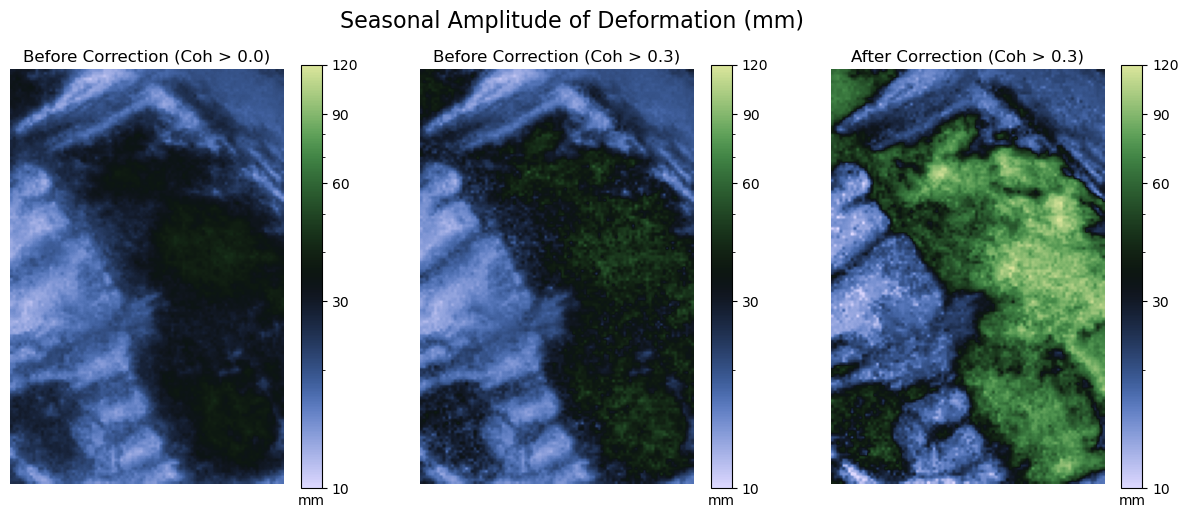
Amplitude retrieval#
For the AnnualSemiannualSinusoidal model, the seasonal amplitude of deformation \(A_{dfm}\) can be calculated by:
where a and b are the coefficients of the annual components sin(T) and cos(T)
amplitude = 2 * np.sqrt(params[0] ** 2 + params[1] ** 2).reshape(n_row, n_col)
amplitude_r = 2 * np.sqrt(params_r[0] ** 2 + params_r[1] ** 2).reshape(n_row, n_col)
amplitude_c = 2 * np.sqrt(params_c[0] ** 2 + params_c[1] ** 2).reshape(n_row, n_col)
import matplotlib.pyplot as plt
from matplotlib.colors import LogNorm

ticks = [10, 30, 60, 90, 120]
norm = LogNorm(vmin=10, vmax=120)

def plot_amplitude(amplitude, ax, title):
    im = ax.imshow(amplitude, cmap=cmaps.tofino, norm=norm)
    ax.axis("off")
    ax.set_title(title)
    # add color bar
    cb = fig.colorbar(im, ax=ax)
    cb.ax.set_yscale("log")
    cb.ax.set_xlabel("mm")
    cb.ax.set_yticks(ticks, labels=ticks)

fig, axs = plt.subplots(1, 3, figsize=(15, 5.5))
plot_amplitude(amplitude_r, axs[0], "Before Correction (Coh > 0.0)")
plot_amplitude(amplitude, axs[1], "Before Correction (Coh > 0.3)")
plot_amplitude(amplitude_c, axs[2], "After Correction (Coh > 0.3)")
fig.suptitle("Seasonal Amplitude of Deformation (mm)", fontsize=16)
plt.show()
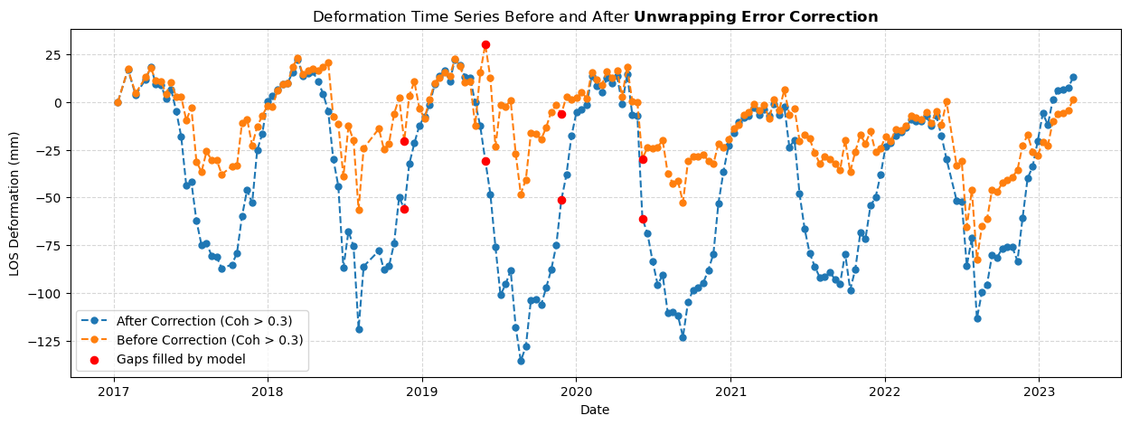
Time series of points#
Retrieve values of points#
For a class inherited from RasterDataset, there is a method row_col() to convert x and y coordinates to row and column index, and xy() to do the reverse. Therefore, we can easily find the row and column index of the given points for a given roi of the dataset.
# set/reset the region of interest (roi) of the dataset
# You can also set the roi when initializing a dataset
ds_unw.roi = roi

# define a point with latitude and longitude
point = query.Points([98.9027314, 38.8218616], crs="EPSG:4326")

# get the row and column of the point in the dataset for given roi
row_col = ds_unw.row_col(point, crs=point.crs)
row_col
array([[48., 81.]])
row, col = row_col[0]
cum_point = cum.reshape(-1, n_row, n_col)[:, row, col]
cum_point_c = cum_c.reshape(-1, n_row, n_col)[:, row, col]
Parse gaps in time series#
Since some pairs may have been masked by the coherence values, there may be some missing values (gaps) have been filled by the time series model. Pairs class provides a method parse_gaps() to find the gaps in the time series by providing the pairs_removed parameter.
Note
Theoretically, the gaps should be the temporal spans (or intervals) between the consecutive acquisitions. For simplicity, the end dates of the gaps will be returned for the parse_gaps() method.
coh_point = coh.reshape(-1, n_row, n_col)[:, row, col]
pairs_removed = pairs_used[coh_point < t_coh]

# parse the gaps caused by the removed pairs
gaps = pairs_used.parse_gaps(pairs_removed)
gaps
array(['2018-11-20T00:00:00', '2019-05-31T00:00:00',
       '2019-11-27T00:00:00', '2020-06-06T00:00:00'],
      dtype='datetime64[s]')
# get the deformation values of the gaps filled by time series model
mask = np.isin(pairs_used.dates[1:], gaps)
gap_vals = cum_point[1:][mask]
gap_vals_c = cum_point_c[1:][mask]
Plot time series of points#
Now we can compare the time series of deformation before and after the unwrapping error correction.
kwargs = dict(linewidth=1.5, ls="--", marker="o", markersize=5)
labels = [
    "Before Correction (Coh > 0.3)",
    "After Correction (Coh > 0.3)",
]

# plot deformation time series
plt.figure(figsize=(15, 5))
plt.plot(pairs_used.dates, cum_point_c, label=labels[1], **kwargs)
plt.plot(pairs_used.dates, cum_point, label=labels[0],  **kwargs)

# plot gaps in deformation time series
kwargs = {"c": "r", "marker": "o", "s": 35, "zorder": 2}
point = plt.scatter(gaps, gap_vals, label="Gaps filled by model", **kwargs)
point = plt.scatter(gaps, gap_vals_c, **kwargs)

plt.legend()
plt.grid(linestyle="--", alpha=0.5)
plt.ylabel("LOS Deformation (mm)")
plt.xlabel("Date")
plt.title(
    "Deformation Time Series Before and After $\\mathbf{Unwrapping\\ Error\\ Correction}$"
)
plt.show()
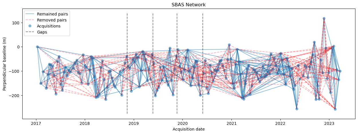
SBAS network visualization#
FanInSAR provides a Baselines class to manage the baselines of the interferometric pairs. You can easily visualize the SBAS network by calling the plot() method.
For the interferogram dataset, there is a parse_baselines() method to parse the Baselines object from the dataset.
bs = ds_unw.parse_baselines(pairs=pairs_used)

fig, ax = plt.subplots(1, 1, figsize=(15, 5))
bs.plot(pairs_used, pairs_removed, ax=ax)
ax.set_title("SBAS Network")
plt.show()
Save results#
For a dataset, you can save the processed results into tiff files by calling the array2tiff() method.
out_file = "/Volumes/Data/GeoData/YNG/Sentinel1/Hyp3/descending_roi/cumulative_deformation.tif"
band_names = pairs_used.dates.strftime("%F")

ds_unw.array2tiff(
    cum_c.reshape(-1, n_row, n_col),
    out_file,
    bounds=roi,
    band_names=band_names,
)
When you open this tiff file in QGIS, you can see the band names are set as the dates of the acquisitions.
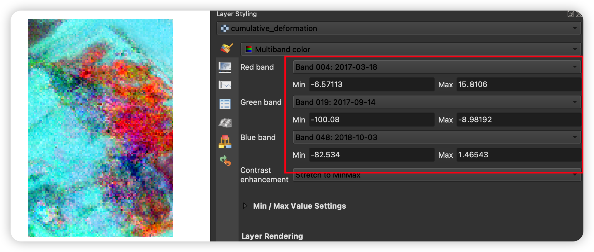
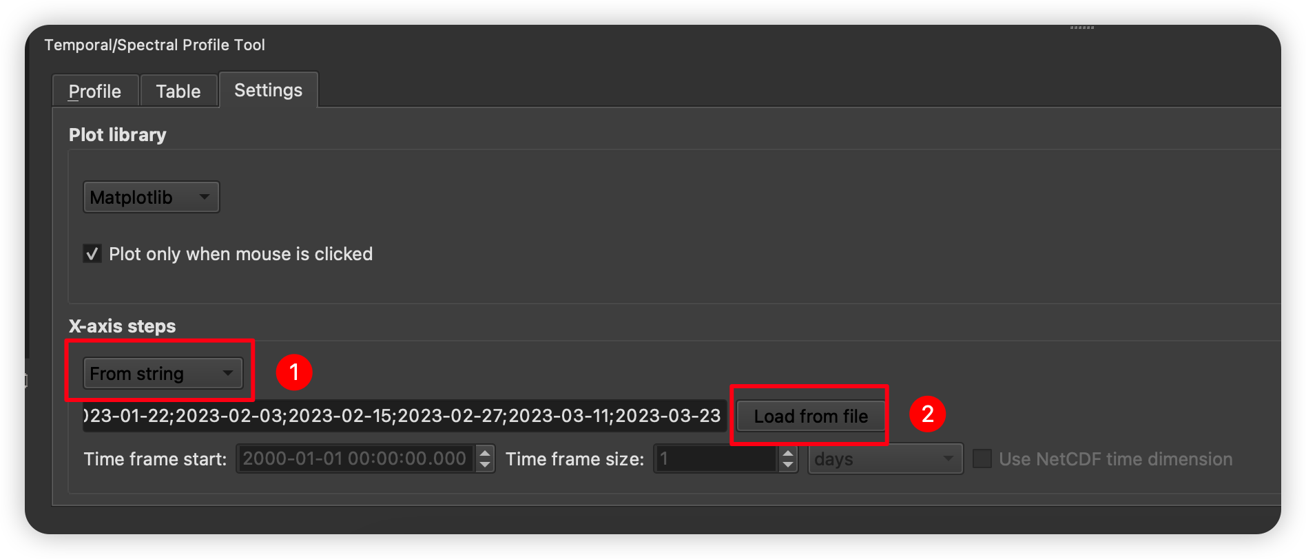
To check the time series of the points, Temporal/Spectral Profile Tool and Value Tool plugins in QGIS are recommended. You can easily install these plugins in QGIS by searching for their names in the QGIS plugin manager.
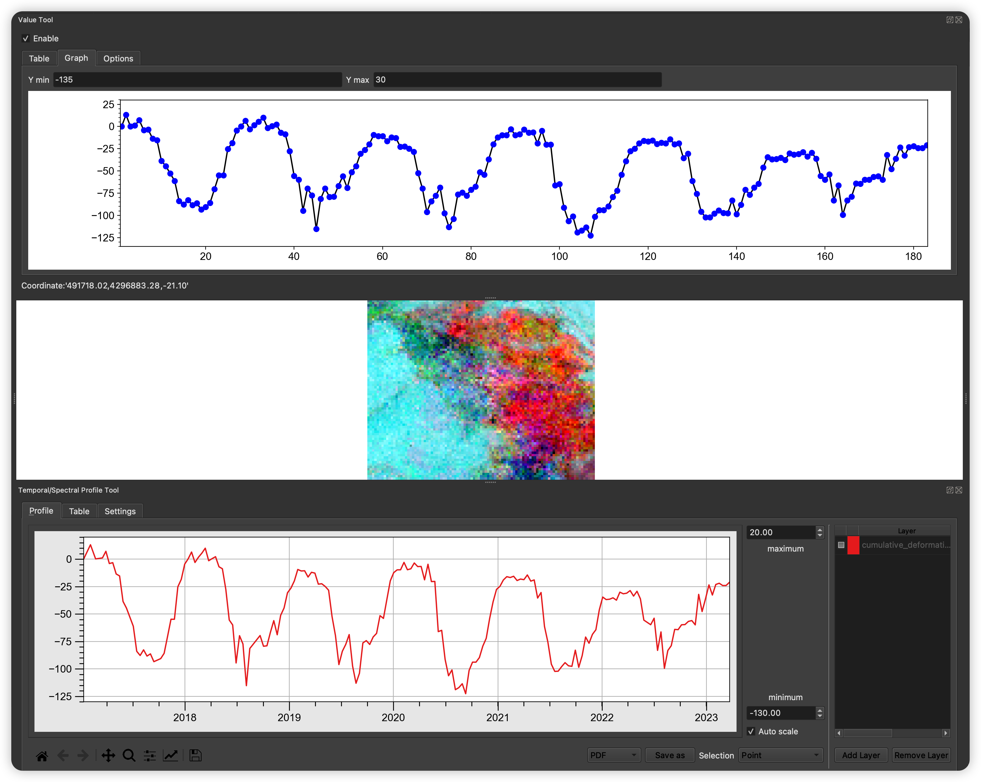
Tip
Temporal/Spectral Profile Tool supports the visualization of the time series with x-axis as time, by changing the x-axis-steps option in the Settings tab to From string.
The band names of tiff file are stored in the corresponding *.band_name.txt file. You can load the date information by clicking the Load from file button.