Custom Time Series Models

In this tutorial, we will discuss how to customize your own time series models in FanInSAR.

from faninsar.NSBAS import TimeSeriesModels
import numpy as np
import pandas as pd
from typing import Sequence, Literal
from datetime import datetime
import matplotlib.pyplot as plt

To create a custom model, you need to inherit from the TimeSeriesModels class. This class is an abstract base class that provides the fundamental framework for time series models. You are required to implement the __init__ method to define model parameters and initialize its state.

For simple mathematical models, it is usually sufficient to specify the observation times (dates) and the time unit (unit). For more complex models, additional parameters may be needed to support the time series modeling.

As an example, we will create a simple cubic deformation time series model. The surface deformation \(d(t)\) is mathematically expressed as:

\[d(t) = a t^3 + b t^2 + c t + d\]

Here, a, b, c, and d are model parameters estimated from NSBAS inversion, and t represents time.

class CubicModel(TimeSeriesModels):
    """Cubic model."""

    def __init__(
        self,
        dates: pd.DatetimeIndex | Sequence[datetime],
        unit: Literal["year", "day"] = "day",
    ) -> None:
        """Initialize CubicModel.

        Parameters
        ----------
        dates : pd.DatetimeIndex | Sequence[datetime]
            Dates of SAR acquisitions. This can be easily obtained by accessing
            :attr:`Pairs.dates <faninsar.Pairs.dates>`.
        unit : Literal["year", "day"], optional
            Unit of day spans in time series model, by default "day".

        """
        super().__init__(dates, unit=unit)
        self._G_br = np.array(
            [
                self.date_spans**3,
                self.date_spans**2,
                self.date_spans,
                np.ones_like(self.date_spans),
            ],
        ).T
        self._param_names = ["Rate of Change", "acceleration", "velocity", "constant"]

1. super().__init__(dates, unit=unit) is used to pass initialization arguments to the parent class TimeSeriesModels. This automatically processes the time series dates and unit, and creates the dates, unit, and date_spans attributes necessary for model construction.

2. date_spans is computed from dates and unit, representing the time span of each date relative to the first date in the series. For simple mathematical models, it is usually sufficient to operate directly on date_spans.

3. self._G_br is used to generate the bottom-right portion of the NSBAS inversion matrix \(G\), which in this case is the matrix \([t^3, t^2, t, 1]\).

4. self._param_names stores the names of the model parameters. We define them as ["Rate of Change", "Acceleration", "Velocity", "Constant"], corresponding to the four coefficients of the cubic model.

dates = pd.date_range("2020-01-01", "2020-12-31", freq="12D")

cubic_model = CubicModel(dates, unit="year")

The model can then be passed to the NSBASMatrixFactory class, which is responsible for constructing the design matrix \(\mathbf{G}\) and data vector \(\mathbf{d}\) used in the NSBAS inversion. For detailed instructions on how to use the NSBASMatrixFactory class, refer to the Operate NSBAS inversion section of the quick start guide.

The bottom-right portion of the NSBAS inversion matrix \(\mathbf{G}\) can be accessed via the G_br method, while the corresponding parameter names are available through the param_names method.

names = cubic_model.param_names
print(names)

['Rate of Change', 'acceleration', 'velocity', 'constant']

print(cubic_model.G_br)

[[0.00000000e+00 0.00000000e+00 0.00000000e+00 1.00000000e+00]
 [3.54628034e-05 1.07939908e-03 3.28542094e-02 1.00000000e+00]
 [2.83702427e-04 4.31759631e-03 6.57084189e-02 1.00000000e+00]
 [9.57495692e-04 9.71459170e-03 9.85626283e-02 1.00000000e+00]
 [2.26961942e-03 1.72703853e-02 1.31416838e-01 1.00000000e+00]
 [4.43285042e-03 2.69849770e-02 1.64271047e-01 1.00000000e+00]
 [7.65996553e-03 3.88583668e-02 1.97125257e-01 1.00000000e+00]
 [1.21637416e-02 5.28905548e-02 2.29979466e-01 1.00000000e+00]
 [1.81569553e-02 6.90815410e-02 2.62833676e-01 1.00000000e+00]
 [2.58523837e-02 8.74313253e-02 2.95687885e-01 1.00000000e+00]
 [3.54628034e-02 1.07939908e-01 3.28542094e-01 1.00000000e+00]
 [4.72009913e-02 1.30607288e-01 3.61396304e-01 1.00000000e+00]
 [6.12797243e-02 1.55433467e-01 3.94250513e-01 1.00000000e+00]
 [7.79117791e-02 1.82418444e-01 4.27104723e-01 1.00000000e+00]
 [9.73099325e-02 2.11562219e-01 4.59958932e-01 1.00000000e+00]
 [1.19686961e-01 2.42864793e-01 4.92813142e-01 1.00000000e+00]
 [1.45255643e-01 2.76326164e-01 5.25667351e-01 1.00000000e+00]
 [1.74228753e-01 3.11946334e-01 5.58521561e-01 1.00000000e+00]
 [2.06819069e-01 3.49725301e-01 5.91375770e-01 1.00000000e+00]
 [2.43239368e-01 3.89663067e-01 6.24229979e-01 1.00000000e+00]
 [2.83702427e-01 4.31759631e-01 6.57084189e-01 1.00000000e+00]
 [3.28421022e-01 4.76014994e-01 6.89938398e-01 1.00000000e+00]
 [3.77607931e-01 5.22429154e-01 7.22792608e-01 1.00000000e+00]
 [4.31475929e-01 5.71002112e-01 7.55646817e-01 1.00000000e+00]
 [4.90237794e-01 6.21733869e-01 7.88501027e-01 1.00000000e+00]
 [5.54106303e-01 6.74624424e-01 8.21355236e-01 1.00000000e+00]
 [6.23294232e-01 7.29673777e-01 8.54209446e-01 1.00000000e+00]
 [6.98014359e-01 7.86881928e-01 8.87063655e-01 1.00000000e+00]
 [7.78479460e-01 8.46248877e-01 9.19917864e-01 1.00000000e+00]
 [8.64902312e-01 9.07774625e-01 9.52772074e-01 1.00000000e+00]
 [9.57495692e-01 9.71459170e-01 9.85626283e-01 1.00000000e+00]]

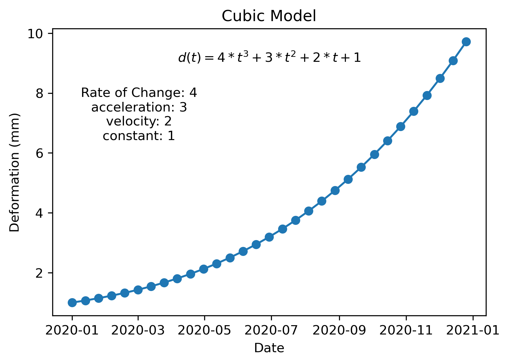
Plotting model deformation

If we get the model parameters \(\mathbf{m}\) after the NSBAS inversion, we can easily calculate the model deformation \(d(t)\) using the \(\mathbf{m}\) vector and the G_br matrix.

m = np.array([4, 3, 2, 1])
d = cubic_model.G_br @ m

plt.figure(figsize=(6, 4), dpi=300)
plt.plot(cubic_model.dates, d, "o-")
plt.text(
    0.2,
    0.7,
    f"{names[0]}: {m[0]}\n{names[1]}: {m[1]}\n{names[2]}: {m[2]}\n{names[3]}: {m[3]}",
    ha="center",
    va="center",
    transform=plt.gca().transAxes,
)
plt.text(
    0.5,
    0.9,
    f"$d(t) = {m[0]} * t^3 + {m[1]} * t^2 + {m[2]} * t + {m[3]}$",
    ha="center",
    va="center",
    transform=plt.gca().transAxes,
)
plt.xlabel("Date")
plt.ylabel("Deformation (mm)")
plt.title("Cubic Model")
plt.show()